
| Distribution tells you the occurence frequency of any particular score in your data; I have talked about this idea in earlier posts. However, today I will look into the different distribution curves that can be used to represent frequency. The essential concept which allows us to make sense of these curves is z-scores. I will show how to calculate those and what they tell about the data. | 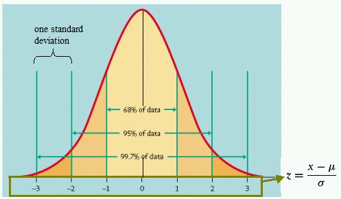 'Normal' distribution |
Normal distribution
Probably the most common distribution shape is Normal, or Gaussian distribution. One of those is pictured above. As you can see, it is a bell-shaped symmetrical curve. Important thing to notice here is that its median = mode = mean, and is represented by its peak; most scores fall within the centre of the curve.
The numbers below are our standard deviations from the mean. The distribution curve does not tell us their value, but shows us their number instead, that is, how far from the mean every score lies.
Other features of Normal Distribution:
1. 68.2% of all the scores fall between -1SD and +1SD from the mean
2. 95.5% of all the scores are between -2SD and +2SD from the mean
3. 99.7% of all the scores are between -3SD and +3SD from the mean
Z-scores
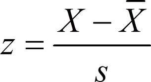
As you might have guessed already, z-score tells us the number of SDs from the mean for each score. Here is the formula to calculate it:
So why do we need to know z value of a score? What useful information does it convey about it?
Apart from showing how typical any particular score is, Z value allows us to see how likely or unlikely it is to occur in our data. For example, we could ask the following question: how likely for a person to score 130 in an IQ test?
All we would need to do is to find a z value for the score of 130, in other words, to find how far from the mean this score would be. The mean of IQs is 100; SD for IQ tests is 15. Thus, following the formula above we get (130-100)/15 = +2.
Likely scores are those which have a z-value between -1.96 and +1.96 (95% scores fall within this spectrum).
Unlikely scores are those which have a z-value below -1.96 or above +1.96, because only 5% of all the scores fall into those categories.
However, you should remember that these apply only when we work with Normal Distribution curve.
Distribution shapes
Distribution curves have two qualities:
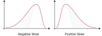
1. Skewness
a) Negative skew - when mean and median are smaller than mode; see below
b) Positive skew - when mean and median are larger than mode; see below.
1. Skewness
a) Negative skew - when mean and median are smaller than mode; see below
b) Positive skew - when mean and median are larger than mode; see below.
2. Kurtosis
a) Kurtosis = 0 in a normal distribution
b) Negative kurtosis - shallow curve
c) Positive kurtosis - steep curve
a) Kurtosis = 0 in a normal distribution
b) Negative kurtosis - shallow curve
c) Positive kurtosis - steep curve
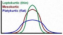
Three kurtosis levels with clever technical labels
