

Chi-square (X^2) is a statistical method used to analyse nominal (frequency) data rather than quantitative data obtained from continuous variables such as height, temperature etc. (scores) and requires between-subjects design. It is used when we want to compare frequency counts of different categories to see whether there is an association between the variables. For example:
- Are gay people more likely to be religious than straight people? (2 variables: religious belief and sexual orientation)
- Are male schoolchildren more likely to pursue academic career in maths than female ones? (variables: gender and programme of choice to study in university).
As always, I will explain the logic of the Chi-Square, show the calculation using an example and talk about Degrees of Freedom and Significance Testing.
Null Hypothesis
In both examples mentioned in the introduction, the data can not be expressed in scores; instead, we simply calculate how many cases fall into each category: females who want to study maths, males who do, females who don't want to study math and females who don't. Then we can present the data in a crosstabulation (or, frequency/contingency table) as follows:
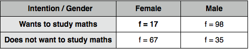
Here, independent variable is two samples (female and male), and dependent variable - intention (2 categories: those who do and those who do not want to study maths). There is a minimum of 2 categories and samples, but can be more; however, it is better to have a few samples and few categories, since large tables can be difficult to interpret. The 'cells' of the table contain the frequencies of individuals from a particular sample who fall in a particular category. For example, in our sample there are 17 female schoolchildren and 98 male schoolchildren who want to study maths.
The statistical question is whether distribution of frequencies in the different samples so varied that it is unlikely that these all come from the same population.
We can see that there are much more boys than girls who want to study maths; these frequencies obtained in a research are called observed frequencies O. However, there is always a possibility that the data came from the same population and that the differences between the samples are only due to the chance fluctuations of sampling (Null Hypothesis). Therefore, we need to see how different each sample is from the population distribution defined by the Null Hypothesis. As ever, we don't have an access to the population data and have to estimate it from the sample characteristics.
Calculation
Firstly, we need to calculate row frequencies R (here, total number of those who want to study maths and total of those who does not), column frequencies C (total number of males and females) and overall frequencies N (total number of cases; 217 in our case):
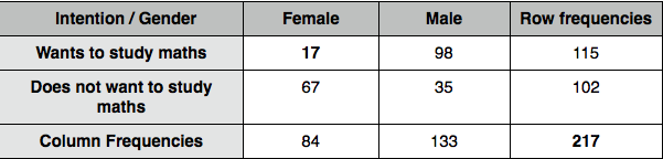
Since under the Null Hypothesis all the differences between the samples are due to chance, we simply combine the samples to get the best estimate of such population. So, in the Null Hypothesis-defined population we would expect approximately 115 out of every 217 schoolchildren to want to study maths in university.
However, there were 17 out of 84 in the first sample and 98 out of 133 in the second sample who wanted to study maths; how do these figures correspond with our population expectations? We need to calculate the expected frequencies E for each of the cells, assuming that the null hypothesis is true (i.e. the nominal variables are unrelated) by using the formula: E = R*(C/N)
So, if Null Hypothesis is true, we would expect 115 out of every 217 female students to have an intention to study maths. Thus, the expected frequency for the first cell is:
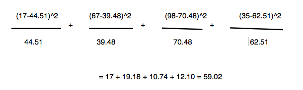
84 * 115/217 = 44.51
Similarly, we would expect 102 out of every 217 to not have an intention to study maths:
84 * 102/217 = 39.48
Following the same procedure, we see that the expected frequency of males who want to study maths is 70.48 and those who don't - 62.51
Next step is to apply the Chi-Square formula:
However, there were 17 out of 84 in the first sample and 98 out of 133 in the second sample who wanted to study maths; how do these figures correspond with our population expectations? We need to calculate the expected frequencies E for each of the cells, assuming that the null hypothesis is true (i.e. the nominal variables are unrelated) by using the formula: E = R*(C/N)
So, if Null Hypothesis is true, we would expect 115 out of every 217 female students to have an intention to study maths. Thus, the expected frequency for the first cell is:
84 * 115/217 = 44.51
Similarly, we would expect 102 out of every 217 to not have an intention to study maths:
84 * 102/217 = 39.48
Following the same procedure, we see that the expected frequency of males who want to study maths is 70.48 and those who don't - 62.51
Next step is to apply the Chi-Square formula:
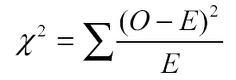
So, lets calculate the Chi-Square for our example:
Degrees of Freedom
Degrees of Freedom for the Chi Square equal (R - 1)(C - 1), where R = numbers of levels in row variable and C = number of levels in column variable. In our case, both variables have 2 levels, therefore (2-1)(2-1) = 1. Note that df do not depend on the sample size as it was in the previous tests.
Significance Testing
Now, all that is left to do is to have a look at the significance table for the Chi Square. As ever, set the p value (normally 0.05) and find the cell opposite our df value. If our X^2 is equal or higher than the critical value, we can reject the H0.
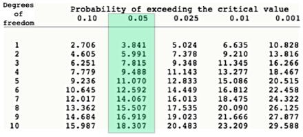
We can see that even with the probability of 0.001, our value of 59.02 is larger than the critical value (10.828), which means we found a significant difference between the frequencies of different samples.
Reporting the results
There was a significant association between gender of schoolchildren and their intention to study maths in university (X^2 = 59.02, df = 1, p < .001). Male schoolchildren were more likely to have an intention to study maths than female children.
Potential troubles; partitioning
1. Expected Frequency in a cell is < 5
In this case, you can not go ahead with the Chi Square test and will have to use Fisher Exact Probability test instead (will be discussed in following posts)
2. Contingency tables with more than 2 categories: partitioning
Sometimes there are more than 2 categories (for example, if we want to compare alcohol consumption among the unemployed, part time and full time working individuals). In this case, expected frequencies, Chi Square and significance testing are carried out in exact same way. df will be bigger than 1 (with 2*3 tables, it will be 2 etc.), so be careful with those.
However, an association between the variables (here, alcohol consumption and employment status) won't tell us where exactly the difference lies. Thus, whenever our df is > 1, we will have to do partitioning: further Chi Squares which would separately test pairs of categories (say, employed full time vs. part time, full time vs. unemployed and part time vs. unemployed).
In this case, we will have to adjust the significance level accordingly. For the three separate Chi Squares our 5% significance level is divided by 3, which gives us a new significance level of 1.67% (0.01).
