

In the previous post I discussed ANOVA for unrelated samples, which is an equivalent of a t-test for unrelated samples. Similarly, within-subjects ANOVA is an equivalent of a t-test for related samples. However, as I stated before, both ANOVAs can be used for comparing more than just two samples.
I will discuss some of the assumptions, explain the logic behind the statistics and show a quick way of calculating the repeated measures ANOVA,
I will discuss some of the assumptions, explain the logic behind the statistics and show a quick way of calculating the repeated measures ANOVA,
Assumptions; sphericity
Once again, the assumptions are pretty much the same that we saw with t-tests for related subjects:
1. Normally distributed data
2. Interval/ratio data
3. Assumption of sphericity
The first two assumptions should be familiar; lets briefly discuss the sphericity. It is similar to homogeneity of variance, which is an assumption of an unrelated t-test. Lets try to understand what the difference is.
In an unrelated t-test we need to make sure that variation of scores of sample 1 is similar to that of sample 2. In other words, that participants in sample 1 differ between each other roughly as much as those in sample 2. This is done to make sure that any differences we find between the samples are due to experimental manipulation and not to other factors.
However, in repeated measures designs there is the added complication that the experimental conditions covary with each other (since it is the same participants who are being tested). The end result is that we have to consider the effect of these covariances when we analyse the data, and specifically we need to assume that all of the covariances are approximately equal (i.e. all of the conditions are related to each other to the same degree and so the effect of participating in one treatment level after another is also equal).
Below I uploaded a Bluffer's Guide to Sphericity by Andy Field. He explains in a fairly simple way what it is, how to measure it and what to do when the assumption is broken. In general, there is no need to worry too much about it, as most of statistics software such as SPSS will tell you if it happens. In such case you would need to use MANOVA - another statistics which I will be discussing later on.
| sphericity.pdf |
Logic behind it
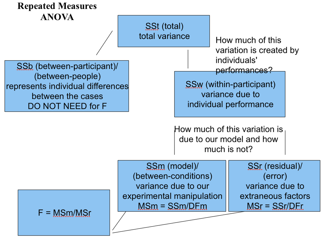
As you remember, in unrelated ANOVA total variance is 'cut' into true and error variance. This is because there is no way to account for individual differences, so we lump them in together with the rest of the error variance. Here, however, error variance can be subdivided by that which can be explained as individual differences and one remaining unexplained.
Getting an estimate of how much contribution to the scores is made by participants' individual characteristics will enable us to revise the error scores so that they no longer contain contribution from individual differences (that is, characteristics which encourage individuals to score generally higher or generally lower on the dependent variable).
Imagine a 'pie' again. One half of it is still 'True variance'; but the second, 'Error', is now divided into two quarters: 'error due to individual differences' and 'Residual Error'.
Link of the logic explained above and the calculation can be expressed in a mind-map like this:
Degrees of Freedom
df[true/between participants] = N[participants] - 1
df[within participants] = N[conditions] - 1
df[residual error] = (N[conditions] - 1) * (N[participants] - 1)
df[within participants] = N[conditions] - 1
df[residual error] = (N[conditions] - 1) * (N[participants] - 1)
Calculation
Now, I will explain the quick method of calculating the ANOVA. The example is taken from the Howitt & Cramer textbook (2008). So, imagine the following scores:
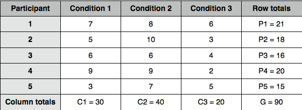
Step 1: calculate total Ex^2 by squaring each score and summing them up:
Ex^2[total] = 49+25+36+81+9+64+100+36+81+49+36+9+16+4+25 = 620
Step 2: calculate the correction factor by dividing squared sum of squares by number of scores:
G^2 / N = 90^2/15 = 540
Step 3: calculate the within-participant sum of squares SS[within]:
SS[within] = C1^2 + C2^2 + C3^2 / number of rows - correction factor = 30^2 + 40^2 + 20^2 / 5 - 540 = 2900/5 - 540 = 580 - 540 = 40
Step 4: calculate the residual error sum of squares SS[error]:
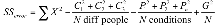
SS[error] = 620 - 580 - 548.667 + 540 = 31.33
Step 5: calculate means of squares (MS) by dividing each SS by appropriate degrees of freedom:
df[within] = N[conditions] - 1 = 3 - 1 = 2
MS[within] = 40 / 2 = 20
df[error] = (N[conditions] - 1) * (N[participants] - 1) = (3-1)*(5-1) = 8
MS[error] = 31.33 / 8 = 3.917
Step 6: calculate F-ratio:
F = MS[within] / MS[error] = 20/3.917 = 5.11
Step 7: calculate the degrees of freedom for between participants variance:
df[between] = N[participants] - 1 = 5 - 1 = 4
Step 8: check for significance. Here, we use the same table that we use for unrelated ANOVA; look for the between and within df in order to find the crucial value. In our case it is 4.459 which is smaller than our result. It means that our samples were taken from different populations. In other words, the means of our samples are significantly different, and we can reject the Null Hypothesis.
