
So far, I mostly talked about the ways to measure a single variable. However, most of statistical operations involve two or more variables; and what the experimenter is normally interested in, is the relationship between those variables. Today, I will talk about the ways to measure and illustrate it.
The relationship between variables can be shown in two different ways: in a scattergram (like that on the right), or with the help of a single numerical index: correlation coefficient. The most common one is Pearson's product-moment correlation coefficient (or simply Pearson's correlation) which contains two pieces of information: 1) the closeness of the fit of the points of a scattergram to the best-fitting straight line through those points and 2) whether the slope of the scattergram positive or negative.
It is important to understand that correlation coefficient does not replace the scattergram entirely, because it omits information about individual scores. However, it neatly summarises a great deal of information and is very useful when comparing several pairs of variables.
Basic Principles
A correlation coefficient consists of two parts:
1. A positive/negative sign (for positive values the sign is frequently omitted)
2. A numerical value from 0.00 to 1.00
Thus, it may look as follows: 1.00; 0.01; -0.50; -0.43; 0.00 etc.
1. The sign +/- tells us the direction of the slope of the correlation line.
a) If the value is positive, it means that the slope is from the bottom left to the top right of the scattergram; it means that the correlation is positive, or, in other words, the value of a variable increases when the value of the other valuable increases.
b) If the value is negative, the slope is from top left to the bottom right of the scattergram; in this case, the correlation is negative. It means that the value of a variable decreases while the value of another variable increases.
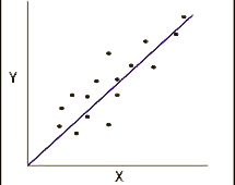 a) Positive Correlation | 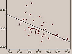 b) Negative Correlation |
2. The numerical value is an index of how close the scores of the scattergram fit the best-fitting straight line.
Thus, a value of 1.00 would mean that all the scores lie exactly on the best-fitting straight line, and we would call it a 'perfect correlation'. A value of 0.00 would mean that all the points of the scattergram are randomly scattered around the straight line, and it is only a matter of pure luck whether any of them actually touches it.
In general, the higher the value is, the closer the points of the scattergram are to the best-fitting straight line.
Therefore, the higher is the value the stronger is relationship between the variables (and the stronger the correlation is).
Another way of thinking about it - it is an index of an amount of variance of the scattergram points from the straight line.
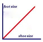 Perfect Positive correlation | 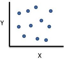 No correlation |
Calculation
Now we know what the correlation coefficient is and what information it carries; but how do we calculate it?
As I mentioned before, the correlation coefficient tells us the joint variance of two variables; something that is called covariance. The calculation of it is almost exactly the same as for variance, but instead of multiplying scores by themselves we multiply the scores of one variable (X) by the scores of another variable (Y).
As I mentioned before, the correlation coefficient tells us the joint variance of two variables; something that is called covariance. The calculation of it is almost exactly the same as for variance, but instead of multiplying scores by themselves we multiply the scores of one variable (X) by the scores of another variable (Y).
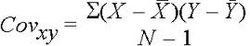
Where X - scores on variable X; X with a dash - mean score on variable X; Y - scores on variable Y; Y with a dash - mean score on the variable Y; N - number of pairs of scores.
Unlike variance, covariance can take positive or negative values; it equals zero if there is no relationship between the variables.
However, the value os covariance is affected by the sizes of variances of each of the variables; the larger they are, the larger is covariance. This makes comparison between pairs of variables quite difficult. The covariance is adjusted by dividing by the square root of the product of the two variances. Once this adjustment is made, we get the formula for the correlation coefficient:
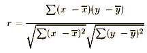
Pearson Correlation Coefficient
Here, the lower part of the formula gives the largest possible value of covariance between the variables (if they are perfectly correlated and their scores lay on a straight line). Dividing the covariance by its largest possible value insures that it can never be higher than 1.00.
Computational formula which does not involve the calculations of the means is as follows:
Computational formula which does not involve the calculations of the means is as follows:
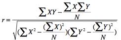
Pearson Correlation Coefficient: computational formula
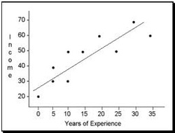
The important point to make in the end is one about outliers: be aware of them and make sure they do not mess your data! It is important to eliminate them BEFORE calculating correlation coefficient, because they can influence it massively. Consider the following scattergram:
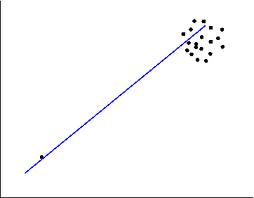
Sneaky outliers messing up the data
It is quite obvious here that one single outlier can give an impression of quite a strong positive correlation, while in fact there is none!
Coefficient of Determination
The r tells us how much variance two variables have in common. However, in order to know precisely how much variance is shared, we need to square it. This squared correlation coefficient is called the coefficient of determination.
Thus, the proportion of variance shared by two variables which have a correlation coefficient 0.40 is 0.40 squared which equals 0.16. To express this in percents, we multiply it by 100% and get 16%. Thus correlation coefficient of 1.00 means that 1.00 squared * 100% = 100% of variance is shared by two variables.
Thus, the proportion of variance shared by two variables which have a correlation coefficient 0.40 is 0.40 squared which equals 0.16. To express this in percents, we multiply it by 100% and get 16%. Thus correlation coefficient of 1.00 means that 1.00 squared * 100% = 100% of variance is shared by two variables.
Spearman's rho
As if it was not enough - there is another correlation coefficient, Spearman's rho (pronounced as 'raw'). basically, it is very similar to Pearson one, but it is used only when the scores are ranked. Instead of taking their value directly from the data, the scores are ranked from smallest to largest. So, the smallest score on variable X is given a rank 1, the second smallest - 2, and so on. Then the Spearman's rho is calculated just like Pearson coefficient between the two sets of ranks - as if the ranks were scores.
Sometimes, however, there are scores with identical values - say, several people could have scored 8 on variable Y. This situation is described as tied scores, or tied ranks. What do we do about them? Conventionally, each of these scores gets an average rank that they would receive if they could be separated.
So, imagine the set of scores: 1, 3, 5, 5, 7, 8, 8, 8, 11. Here we have two scores of 5. If they could be separated by some fractional amount, we would give them ranks 2 and 3 accordingly. However we can not separate them, so we give them the average of these ranks: 2.5 each ((2+3)/2 = 2.5).
You might have noticed that we have three scores of 8; we deal with them in just the same way. If they were slightly different, they would be ranked 6, 7 and 8; however, we allocate the average of these ranks to each of them - which in this case is 7 ((6+7+8)/3 = 7). The next score gets the rank 9.
Thus, we will have a following table of scores and their ranks:
1 3 5 5 7 8 8 8 11
1 2.5 2.5 4 5 7 7 7 9
You might be wondering now - why even bother converting the scores into ranks???
The answer is, it is traditionally used when distributions of scores on a variable are very unsymmetrical and are very distorted from a normal distribution. Otherwise, I would recommend to stay away from ranks - correlation coefficients are painful enough without them!
